The art and science of hyperparameter optimization on Amazon Nova Forge

Large language models (LLMs) deliver strong results on general tasks, but they often struggle with specialized work that requires understanding proprietary data, internal processes, or domain-specific terminology. Amazon Nova Forge addresses this by enabling you to build your own frontier models using Amazon Nova. You can start development from early model checkpoints, blend proprietary data with Amazon Nova-curated training data, and host custom models securely on AWS. A key capability is data mixing, which blends your training data with curated datasets. This helps the model absorb your domain while retaining broad reasoning, instruction-following, and language capabilities. This prevents catastrophic forgetting that typically undermines domain customization.

Successful customization requires careful hyperparameter tuning. Learning rate, data mixing ratio, checkpoint selection, and training techniques all interact in ways that can silently undermine a training run. If any of them are wrong, you trade one problem for another. This post covers the art (strategic trade-offs) and science (metric-driven decisions) of hyperparameter tuning on Amazon Nova Forge to help you avoid expensive failed training runs.

Fine-tuning for domain-specific tasks means improving performance in one area without degrading the model’s general capabilities, and getting that balance right is harder than it looks. This post walks through how to navigate that balance, from selecting the right customization strategy for your data and task, to configuring the training parameters that most influence outcomes, like learning rate, batch size, and checkpointing. We also cover the common mistakes that lead to wasted training runs and how to catch them early, so you can improve domain performance without degrading general capabilities or burning through compute on avoidable failures.

By the end, you will know how to improve domain performance without degrading general capabilities and how to avoid the expensive failures that come from getting the balance wrong.

The hyperparameter tuning challenge

Achieving this balance is harder than it appears. Three fundamental challenges make hyperparameter tuning particularly difficult on domain-specialized models.

Challenge 1: Catastrophic forgetting

When you train a model on narrow domain data, the model can overwrite general capabilities it learned during pre-training. This phenomenon, called catastrophic forgetting, shows up as degraded performance on tasks outside your training domain. The model becomes highly specialized but loses instruction-following ability, reasoning capability, and broad knowledge. In production, this means a customer service model fine-tuned on your support tickets may no longer reason about ambiguous requests or maintain coherent multi-turn conversations.

This creates a stability-flexibility tradeoff. Ideally, the model is flexible enough to learn about an organization’s domain but stable enough to retain general capabilities. Nova Forge addresses this through data mixing, which blends your training data with curated datasets during training, and checkpoint selection, which lets you choose how much existing alignment to preserve.

Challenge 2: Finding the right learning rate

The learning rate controls how much the model’s weights change in response to each batch of training examples. It’s the most sensitive hyperparameter across all customization techniques. A learning rate that’s too high causes the model to overshoot the optimal state, destabilize during training, or forget base capabilities rapidly. A learning rate that’s too low wastes compute on very slow convergence. The right value depends on your data distribution, mixing ratio, and training technique.

Nova Forge provides calibrated service defaults for each training technique that account for these interactions. When you use data mixing, the sensitivity increases further. Deviating from the default learning rate when mixing Nova data with your own data is the most common source of training instability, so these service defaults are the recommended starting point.

Challenge 3: Baseline performance constraints

Reinforcement fine-tuning (RFT) is a technique that improves model behavior by generating multiple candidate responses and scoring them against quality criteria. The model learns by comparing its own outputs and reinforcing the better ones. RFT works at its full capacity within a specific range of baseline task accuracy, measured by how often the model produces correct or high-quality responses before fine-tuning. If baseline accuracy is too low (the model rarely produces correct responses), there aren’t enough good examples for reward-guided exploration to learn from. If baseline accuracy is already very high, additional training yields diminishing returns and risks degrading existing performance. This means RFT can’t close large competence gaps where the model fundamentally lacks the knowledge or reasoning ability to attempt a task. It refines and strengthens behaviors the model can already partially demonstrate, rather than teaching entirely new capabilities from scratch.

The Nova Forge pipeline addresses both bounds. For low-baseline scenarios, run supervised fine-tuning (SFT) first to establish the foundational capabilities needed for effective reward-based learning. For high-baseline tasks, make sure that your reward function has discriminative power across the model’s quality range. If most responses already score highly, RFT has no meaningful signal to optimize against.

The Nova Forge customization pipeline

Understanding these challenges frames how the Amazon Nova Forge customization pipeline is designed to address them. Nova Forge provides three complementary customization techniques, each serving a distinct purpose in the model development lifecycle.

Technique	What it does	When to use	Input data
Continued pre-training (CPT)	Expands foundational model (FM) knowledge through self-supervised learning on large quantities of unlabeled, domain-specific proprietary data. CPT teaches the model domain terminology and patterns from your text corpus.	You need the model to understand specialized vocabulary, industry concepts, or organizational knowledge that does not exist in the base model.	Large volumes of unlabeled domain text. Nova Forge supports CPT with data mixing and three checkpoint options (pre-trained, mid-trained, and post-trained), each suited to different data scales and downstream requirements.
Supervised fine-tuning (SFT)	Customizes model behavior using a training dataset of input-output pairs specific to your target tasks. SFT teaches the model “given X, output Y” behavior through demonstrations.	You need the model to follow specific response formats, adopt particular tones, or perform structured tasks like classification or extraction.	1,000–10,000 high-quality demonstrations per task. Quality, consistency, and diversity matter more than volume. Nova Forge supports SFT with data mixing using Amazon Nova-curated datasets, including reasoning-instruction-following categories that preserve general capabilities.
Reinforcement fine-tuning (RFT)	Steers model output toward preferred outcomes using reward signals. RFT optimizes the model within a behavioral neighborhood established by prior training for single-turn or multi-turn conversational tasks.	You have a clear reward function that can evaluate response quality and want to push performance beyond what SFT alone achieves.	Prompts and a reward function. Nova Forge supports bringing your own external reward environment through AWS Lambda, enabling custom verification logic for domain-specific quality assessment.

When all three stages are used together (CPT, then SFT, then RFT), they produce the strongest results. However, with the right pipeline, each stage can be optional. It depends on your data availability, task type, and starting point. CPT is only needed when the base model lacks domain vocabulary or knowledge your task requires. SFT and RFT can be used independently or combined depending on what your task demands.

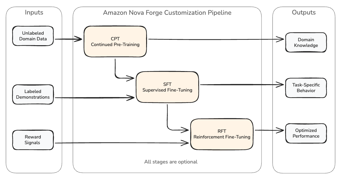
Figure 1: The Amazon Nova Forge customization pipeline. CPT teaches domain knowledge from unlabeled text, SFT teaches task-specific behavior from demonstrations, and RFT optimizes performance using reward signals. Each stage is optional, and the full pipeline (CPT, then SFT, then RFT) produces the strongest results when all three are applicable to your use case.

Amazon SageMaker AI offers different environments for customization: SageMaker Serverless provides a UI-driven experience with automatic compute provisioning, SageMaker AI training jobs (SMTJ) provide a fully managed experience without cluster management, while Amazon SageMaker HyperPod offers specialized environments for advanced distributed training scenarios.

Strategic decisions

With the customization pipeline in view, the next step is understanding the qualitative trade-offs that shape your configuration. These strategic decisions matter as much as any individual hyperparameter value: checkpoint selection, data mixing, and training mode.

Checkpoint selection (most impactful decision)

For CPT, checkpoint selection is more impactful than any hyperparameter. Amazon Nova Forge provides three checkpoint options, each suited to different data scales and downstream requirements.

Pre-trained checkpoints are the most flexible and offer the fastest convergence. These checkpoints accept new patterns readily and work best for large-scale CPT with substantial token budgets exceeding 100 billion tokens. When using pre-trained checkpoints with large datasets, you can use a higher learning rate (such as 1e-4) to accelerate knowledge absorption. You then need to gradually reduce the learning rate back to approximately 1e-6 for model stability before running SFT to let the model “settle” into what it learned without overshooting. Be aware that pre-trained checkpoints have no instructions for tuning. After CPT, you must run SFT to make the model useful for downstream tasks.
Mid-trained checkpoints balance flexibility and alignment. They accept domain knowledge while retaining some instruction-following behavior. Use mid-trained checkpoints for medium-sized datasets where you want faster domain adaptation than post-trained but more stability than pre-trained. Mid-trained checkpoints work well for full rank training, which updates every parameter in the model during fine-tuning, with large, structured datasets.
Post-trained checkpoints are the most resistant to new patterns but preserve instruction-following and general capabilities. Use post-trained for smaller-scale CPT where preserving alignment matters more than maximizing domain knowledge absorption. Post-trained checkpoints are the recommended starting point for LoRA (Low-Rank Adaptation), which freezes the original model weights and trains small adapter matrices on top, and other parameter-efficient fine-tuning methods, as they maintain the model’s existing capabilities while allowing targeted adaptation. For small datasets or later-stage checkpoints, use conservative learning rate values from the service defaults.

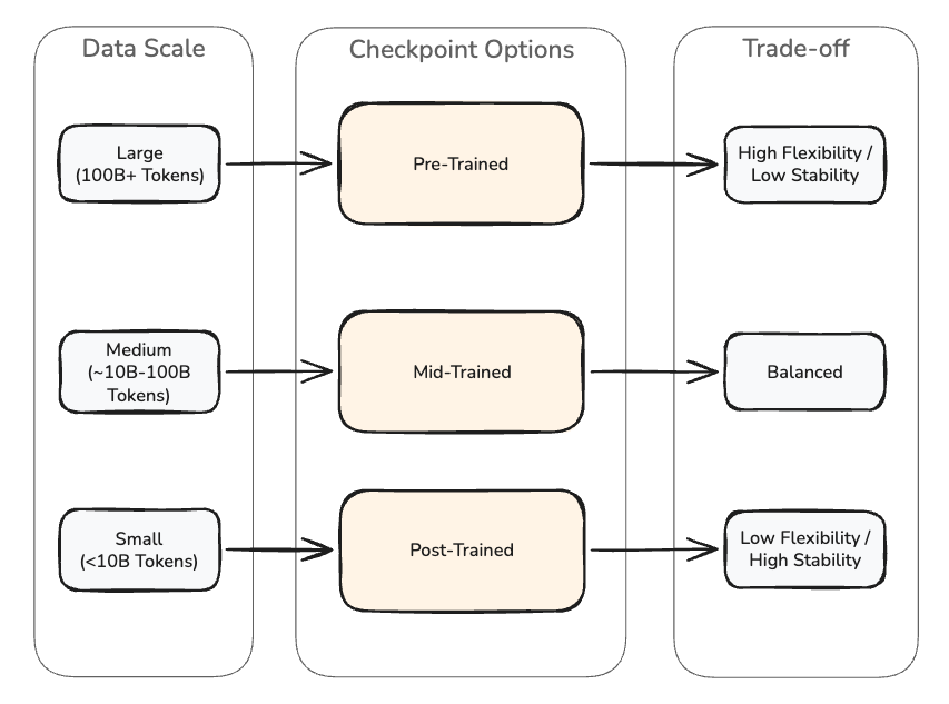
Figure 2: Checkpoint selection for continued pre-training. Pre-trained checkpoints offer maximum flexibility for large datasets but require SFT afterward to restore instruction-following. Post-trained checkpoints preserve alignment and suit smaller datasets or parameter-efficient methods like LoRA.

Data mixing strategy

Without data mixing, training on narrow domain data can cause the model to become unstable, resulting in erratic training behavior (gradient instability or loss spikes) or a sudden degradation in performance.

When configuring data mixing, balance your customer data around 50 percent of the total mix for most use cases. For SFT, always include the “reasoning-instruction-following” category in your Nova data mix. This single category significantly improves generic benchmark performance after fine-tuning. Skipping this category is a common cause of degraded reasoning performance in fine-tuned models.

Data mixing is very sensitive to learning rate. Deviating from the default learning rate when using data mixing causes instability. This is the most common mistake practitioners make. If you observe training instability with data mixing, the learning rate is the first suspect.

Finding the optimal mixing ratio requires experimentation. Hold your domain data constant and vary the Nova data proportion across several runs. Domain performance typically stays constant while general capabilities keep improving the more Nova data is mixed in. Place your highest-quality data toward the end of training for better convergence.

Training mode: Low-Rank Adaptation (LoRA) vs Full Rank

Amazon Nova Forge supports two training modes that determine how model parameters are updated during training:

LoRA updates only adapter layers, offering lower compute costs, faster iteration, and compatibility with on-demand inference. LoRA achieves near Full Rank performance for most tasks while being more forgiving of suboptimal hyperparameters. The default alpha scaling factor of 64 works for most tasks. Increase alpha if LoRA is under-adapting to your data or decrease it if LoRA is over-adapting and losing general capabilities. Use post-trained checkpoints as your starting point for LoRA training.
Full Rank updates all model parameters, providing maximum adaptation capacity. Full Rank requires Amazon Bedrock Provisioned Throughput for deployment (On-Demand is only available for LoRA-based customization) and higher compute during training. Use Full Rank when you have validated your pipeline and your deployment architecture justifies the additional cost. Mid-trained checkpoints work well for Full Rank training with large, structured datasets.

Start with LoRA to validate your pipeline, data quality, and reward function (for RFT). Graduate to Full Rank when you have confirmed the approach works, and your production requirements justify it (for example, model performance or cost constraints).

Recommended workflow

Applying these strategic decisions to your specific situation depends on what data and objectives you have. The following paths map your starting conditions to the right sequence of techniques.

If you have labeled demonstrations and a verifiable reward function (SFT then RFT):

Start with SFT using LoRA to teach the target behavior and establish baseline competency.
Enable data mixing with “reasoning-instruction-following” included to preserve the model’s ability to follow structured prompts and produce well-formatted outputs during domain adaptation.
Use default learning rates without modification.
Monitor validation loss to select the best SFT checkpoint.
Graduate to RFT on the SFT checkpoint to optimize further through reward signals.
Consider Full Rank training only after validating the approach with LoRA.
Test thoroughly on both your domain task and general benchmarks before production deployment (see the Experiments and insights section for an example).

If you can define verifiable outcomes but cannot easily label responses at scale (RFT only):

Evaluate base model performance on a representative sample of your task first.
Proceed with RFT directly if the base model achieves more than approximately 5 percent positive reward.
Fall back to SFT if reward scores are consistently near zero. The model needs baseline competency before reward-guided learning can take effect.

If the base model lacks domain vocabulary or knowledge your task requires, start with CPT:

Run CPT to absorb domain knowledge from unlabeled text.
Follow with SFT. Pre-trained checkpoints used for CPT have no instruction tuning, so SFT is required after CPT to make the model useful.
Optionally follow with RFT to further optimize performance.

Parameter configuration

With strategic decisions made, you can now optimize specific hyperparameters that govern how each technique executes. This section provides guidance for each technique.

Learning rate configuration

Learning rate controls how quickly the model updates based on training signals. Service defaults represent tested configurations that work across diverse use cases.

For CPT: Start at service defaults. For large datasets exceeding one trillion tokens, you can use a higher learning rate (such as 1e-4) to accelerate knowledge absorption, but you need a ramp-down stage to reduce the learning rate back to approximately 1e-6 for model stability before SFT. The constant_steps parameter controls how many steps the model trains at the peak learning rate before this ramp-down stage begins. Increase constant_steps for very large token runs where more steps at full learning rate help domain absorption. For smaller datasets or later-stage checkpoints, use the default (lower) learning rate from the start.
For SFT: Stick to service defaults, especially with data mixing. The recommended learning rate is 1e-5 for LoRA and 5e-6 for full-rank SFT. Deviating from the default learning rate when mixing Nova data causes instability. If you observe training instability with data mixing, the learning rate is the first suspect.
For RFT: Start at service defaults. Adjust in small multiplier increments only if needed. If reward drops suddenly and does not recover, the learning rate is likely too high. Even a small multiplier increase can drop performance below baseline.

Configure warmup steps to approximately 15 percent of your total training steps. Warmup stabilizes initial training by gradually increasing the learning rate rather than starting at the full value.

Batch size and training duration

Batch size (controlled by global_batch_size) is the batch parameter across all training methods (CPT, SFT, RFT) and all environments (SageMaker Serverless, SMTJ, HyperPod). It defines the number of training samples processed per optimizer step. For CPT and SFT, this is straightforward with one sample equal to one input-output pair (SFT) or one token sequence (CPT). RFT introduces an additional parameter, number_generation, that controls how many candidate responses are generated per prompt for reward scoring. This parameter doesn’t exist in CPT or SFT recipes, because those methods train directly on provided input-output pairs rather than generating candidates. When the number of generations parameter is present, batch size semantics differ between environments. Getting this wrong leads to unexpected behavior.

On SMTJ (RFT only): Batch size means prompts per step. Each prompt generates N candidate responses (controlled by number_generation). Total samples per step equals batch size multiplied by number of generations.
On SageMaker HyperPod (RFT only): Batch size means total samples per step (prompts multiplied by generations). Translate carefully when moving configurations between environments.

For CPT, target 2-20 million tokens per step. Use 20 million for large token budgets and 2 million for smaller budgets. Calculate global batch size as the nearest power of 2 of tokens per step divided by max sequence length. For example, 4 million tokens per step with a 4096-sequence length yields a batch size of approximately 1024. Smaller batch sizes produce noisier gradients, which can help generalization and enable faster iteration. Larger batch sizes produce smoother gradients but may over-smooth domain-specific signals. Start with moderate batch sizes for stability.

Match your max sequence length to your data distribution. Don’t exceed what your data needs. Smaller context lengths increase token throughput and reduce training costs. For CPT, process at most one epoch of your dataset. Avoid repeating data, as multiple epochs on limited CPT data leads to overfitting and loss of general capabilities. Monitor validation loss to track progress. For SFT, Full Rank training typically needs fewer epochs than LoRA. LoRA training can tolerate slightly more epochs. Monitor validation loss to detect overfitting and select the best checkpoint.

RFT-specific parameters

RFT introduces additional parameters not present in CPT or SFT.

Number of generations controls how many candidate responses the model generates per prompt for the reward function to compare. Fewer candidates mean faster training but less signal diversity. Too many candidates add noise without improving signal and nearly double training time. Moderate values hit the best accuracy-to-time ratio. Increase if your task has high variance in response quality. Decrease for rapid reward function iteration during development.
KL-Divergence Loss Coefficient constrains how far the model’s policy can drift from its original behavior. This parameter is available on SMTJ only. A low coefficient lets the model explore freely but risks finding shortcuts that game the reward function. A high coefficient prevents meaningful learning by pulling the model back to its starting point. Increase if KL divergence spikes during training to balance genuine learning against behavioral drift.
Reasoning Effort controls how much chain-of-thought reasoning the model performs before answering. High reasoning effort produces the best accuracy but increases latency and serving cost. Low reasoning effort offers faster inference with modest accuracy trade-offs. Use high for maximum accuracy during validation, then consider reducing for latency-sensitive production deployments.
Lambda Concurrency Limit (SMTJ only) controls parallel AWS Lambda functions for reward evaluation. Increase significantly for fast reward functions to avoid evaluation throughput becoming a bottleneck.

Remember that batch size semantics differ between platforms. On SMTJ, global_batch_size means prompts per step where each generates N candidates. On SageMaker HyperPod, global_batch_size means total samples (prompts multiplied by generations). Translate carefully between environments.

Regularization parameters

Regularization parameters help prevent overfitting, especially on smaller datasets.

Weight decay defaults to zero. Increase modestly if you observe overfitting on small datasets. Weight decay applies L2 regularization to constrain parameter magnitudes.
Dropout (hidden and attention) defaults to zero. Increase hidden dropout modestly for smaller datasets to reduce overfitting. Increase attention dropout cautiously, as high values can hurt complex reasoning capabilities.
Clip ratio and age tolerance are advanced SageMaker HyperPod parameters. Clip ratio limits how much the policy can change in a single training step. Age tolerance determines how long training data remains valid before being considered too stale. Refit frequency controls how often the model collects fresh training data. Defaults work for most use cases. Only adjust these advanced settings if you understand the specific stability issue you are addressing.

Experiments and insights

With these hyperparameters in mind, we ran a series of HPO experiments using Amazon Nova 2.0 across public benchmarks including CoCoHD, MedReason and LLaVA-CoT. The following table summarizes the experimental configurations and key findings for each parameter sweep.

Dataset	Rank	Alpha	GBS	LR	Max Steps	Warmup	Base Target Perf.	SFT Target Perf.	Rank	Perf Diff
MedReason	32	64	32	1.00E-05	312	47	57.38%	63.54%	2	10.75% ↑
MedReason	64	64	32	1.00E-05	312	47	57.38%	63.78%	1	11.16% ↑
MedReason	32	64	32	5.00E-06	312	47	57.38%	63.33%
MedReason	32	64	32	1.00E-05	624	94	57.38%	61.42%
LLavaCOT	64	64	32	1.00E-05	312	47	16.22%	68.47%	1	322.13% ↑
LLavaCOT	32	128	32	1.00E-05	312	47	16.22%	65.77%	2	305.49% ↑

We ran LoRA SFT on Amazon Nova 2 Lite using Nova Forge with rank 32, alpha 64, batch size 32, 15 percent warmup, and 1 epoch, sweeping only the learning rate to isolate its effect on target accuracy. The service default of 1e-5 produced the best result at 63.54 percent, a 10.75 percent lift over the v4 base. Dropping the learning rate to 5e-6 adversely impacted target performance without meaningfully protecting general capabilities, as MMLU, IFEval, and GPQA scores were within noise of the 1e-5 run. Doubling to 2 epochs at the same learning rate dropped accuracy to 61.42 percent, confirming that overtraining on narrow domain data erodes both domain and general performance.

We varied LoRA rank (32 vs 64) and alpha (64 vs 128) on a multimodal reasoning task where the base model starts at only 16.22 percent accuracy. The best configuration, rank 64 with alpha 64, lifted accuracy to 68.47 percent, a 322 percent relative improvement over the base. Doubling alpha to 128 at rank 32 produced a similar target gain at 65.77 percent, but at a meaningfully higher general-capability regression cost. For tasks where the baseline accuracy is low, increasing rank is a higher-leverage adjustment than increasing alpha. Alpha should be increased only when LoRA is under-adapting, and decreased if the model is losing general capabilities.

No single hyperparameter configuration works best for all use cases. These recommended defaults are strong starting points, not guarantees of optimal performance.

Common pitfalls and how to avoid them

The following table summarizes the most common mistakes practitioners should avoid when tuning Amazon Nova Forge models.

Pitfall	Symptom	Solution
Skipping SFT before RFT	RFT produces no improvement or degrades performance	Run SFT first to get the model into the right behavioral neighborhood before RFT optimization.
Deviating from default LR with data mixing	Training instability, loss spikes, capability collapse	Stick to service defaults when using data mixing. This is the most common mistake.
Poor reward function quality	Accuracy decreases despite training, or model games the metric	Refine your reward function before changing any training parameter. Validate with at least two independent judges.
Multiple epochs on limited CPT data	Overfitting, loss of general capabilities, memorization	Process at most one epoch of your CPT dataset. Monitor validation loss to detect overfitting early.
Mismatched reasoning settings	Inference behavior does not match training behavior	Match `reasoning_enabled` between training and inference. If you train with reasoning, infer with reasoning.

When tuning models with Nova Forge, invest in your reward function before anything else. A poor reward function will decrease accuracy regardless of other hyperparameter choices, while a refined one produces consistent gains on identical infrastructure. Make sure your reward function has discriminative power across the model’s quality range, because if everything scores high, RFT has no gradient to optimize.

The same validation discipline applies to LLM-as-judge selection. Your judge model must reliably distinguish quality differences across the model’s output range. Validate judge agreement with at least two independent evaluators before committing to a training run.

Be aware that training environment stability mechanisms differ between platforms. SMTJ applies continuous KL penalty as a soft constraint, while SageMaker HyperPod uses gradient clipping as a hard cap per step. Both achieve comparable accuracy, but they require different tuning intuitions. Do not assume parameters transfer directly between environments.

Throughout all of this, prioritize data quality over volume. Filtering aggressively and making sure training examples accurately represent the target behavior will outperform simply scaling up low-quality data.

Measuring success

When you apply proper hyperparameter tuning, the results can be substantial. The AWS China Applied Science team demonstrated this in their evaluation of Amazon Nova Forge, achieving 17 percent F1 score improvement on a complex Voice of Customer classification task while maintaining near-baseline MMLU scores.

Key metrics to monitor

Training loss should decrease steadily without sudden spikes. Spikes often indicate learning rate issues or data quality problems.

Validation loss reveals overfitting. If validation loss increases while training loss decreases, you are overfitting. Reduce epochs, increase regularization, or add more diverse data.

KL divergence (for RFT) shows how far the policy has drifted. Sudden spikes suggest the model is making large, potentially unstable updates. Increase the KL loss coefficient if this occurs.

Reward metrics (for RFT) should improve steadily. If reward improves rapidly then plateaus or drops, the model may be gaming the reward function. Revisit your reward design.

Conclusion

Optimizing model customization with Amazon Nova Forge requires balancing art and science. The art involves understanding trade-offs: checkpoint selection, data mixing strategy, and training mode decisions shape your outcome more than any single hyperparameter. The science involves systematic tuning: learning rate, batch size, and technique-specific parameters require careful configuration based on your data and objectives.

Data and reward quality exceed any hyperparameter in importance. Before tuning training parameters, optimize your data pipeline and reward function. Start with service defaults, especially for learning rate and data mixing, as these defaults exist because they work across a wide range of use cases.

For most production scenarios, the strongest pipeline is SFT followed by RFT. RFT refines existing capability but cannot recover from a low baseline, so supervised fine-tuning needs to establish solid performance first. Data mixing should be treated as essential for production workloads, not optional. It prevents catastrophic forgetting and provides optimization stability needed for reliable results.

When working with continued pre-training, checkpoint selection is the most impactful decision you will make. Match checkpoint flexibility to your data scale: earlier checkpoints for large-scale domain adaptation, later checkpoints for smaller datasets where preserving instruction-following behavior matters.

To get started with Amazon Nova Forge, explore the Amazon Nova documentation and the SageMaker HyperPod recipes repository on GitHub. For hands-on examples of data mixing in action, see the Nova Forge data mixing blog post. For a deeper dive into RFT with Nova Forge see the Reinforcement fine-tuning for Amazon Nova: Teaching AI through feedback blog post.

Acknowledgements

The authors would like to thank Zheng Du, Bharathan Balaji, Anjie Fang, and Mengnong Xu from the AWS AGI Customization Science team for their technical guidance.