Optimize model training on Amazon SageMaker AI with NVIDIA Blackwell

Optimizing model training on Amazon SageMaker AI with NVIDIA Blackwell GPUs changes what’s practical for large AI models. If you train large models today, you are likely working around a familiar set of constraints: batch sizes limited by GPU memory, sequence lengths cut short to avoid out-of-memory errors, and model sharding that adds communication overhead as you scale. Blackwell’s expanded memory and new precision formats reduce those constraints directly. P6-B200 instances with 8 Blackwell GPUs are available on Amazon SageMaker AI Training jobs, and you can book the capacity using Flexible Training Plan with predictable access, cost management, and automated resource management. Amazon SageMaker AI training jobs let you train ML models at large scale by automatically provisioning and managing the underlying compute infrastructure and resources, so you can focus on your data and algorithms rather than infrastructure operations.

This post shows you how to configure training jobs on Amazon SageMaker AI to get the most out of Blackwell’s architecture on AWS. You learn how to select batch sizes and sequence lengths that take advantage of Blackwell’s expanded memory, choose the right precision format for your model size (1B to 64B parameters), and apply activation checkpointing strategically. By the end, you have a practical framework for tuning your training configuration and launching distributed training jobs on P6-B200 instances.

Properly configured Blackwell training jobs can process larger batch sizes without aggressive sharding, reducing communication overhead and improving throughput. Longer sequence lengths become viable for long-range dependency tasks. With the right precision format, models that previously required multi-node setups can run on a single 8-GPU node, which means faster iteration cycles, less networking overhead, and lower infrastructure costs.

Understanding NVIDIA Blackwell

Before you configure your training job, it helps to understand what makes Blackwell different from previous GPU generations. Blackwell’s dual-chip architecture and fifth-generation Tensor Cores deliver measurable gains for multi-GPU training out of the box. The NVLink 5 interconnect provides up to 1.8 TB/s of bidirectional GPU-to-GPU bandwidth, while B200’s larger HBM capacity and higher memory bandwidth help reduce memory pressure for large batches, long sequences, and distributed training workloads.

The examples in this post use single-node 8-GPU training with transformer models ranging from 1B to 64B parameters. The training configuration uses PyTorch Fully Sharded Data Parallel (FSDP), a distributed training technique that shards model parameters, gradients, and optimizer states across GPUs to train models larger than single-GPU memory. The results cover multiple configurations with varying batch sizes, sequence lengths, and precision formats to show when different approaches deliver the optimal results.

Memory management

Blackwell’s expanded memory (180 GB on B200, 268 GB on B300) gives you room to optimize in three areas: larger batch sizes, simplified model sharding, and longer sequence lengths.

Larger batch sizes reduce the number of gradient synchronization steps across GPUs, improving overall throughput.
Simplified model sharding becomes possible because more memory per GPU means you might be able to reduce the degree of model parallelism or eliminate it entirely for some models. Fewer shards mean less inter-GPU communication overhead.
Longer sequence lengths allow models to process more context in a single pass, which is critical for long-range dependency tasks.

If throughput is your primary goal, start with batch size tuning. If communication overhead is the bottleneck, simplify sharding first. If your task requires long-range context, prioritize sequence length. Batch size and sequence length both increase memory consumption and finding an effective balance matters.

Activation checkpointing helps you balance memory use and compute. It trades increased compute time (typically 10-30% overhead depending on model architecture) for a reduction in GPU memory usage by recomputing intermediate activations during the backward pass instead of storing them. The freed memory can then be reinvested into larger batch sizes or longer sequences. Since the compute overhead varies by workload, benchmark your specific configuration to understand the trade-off before committing to checkpointing.

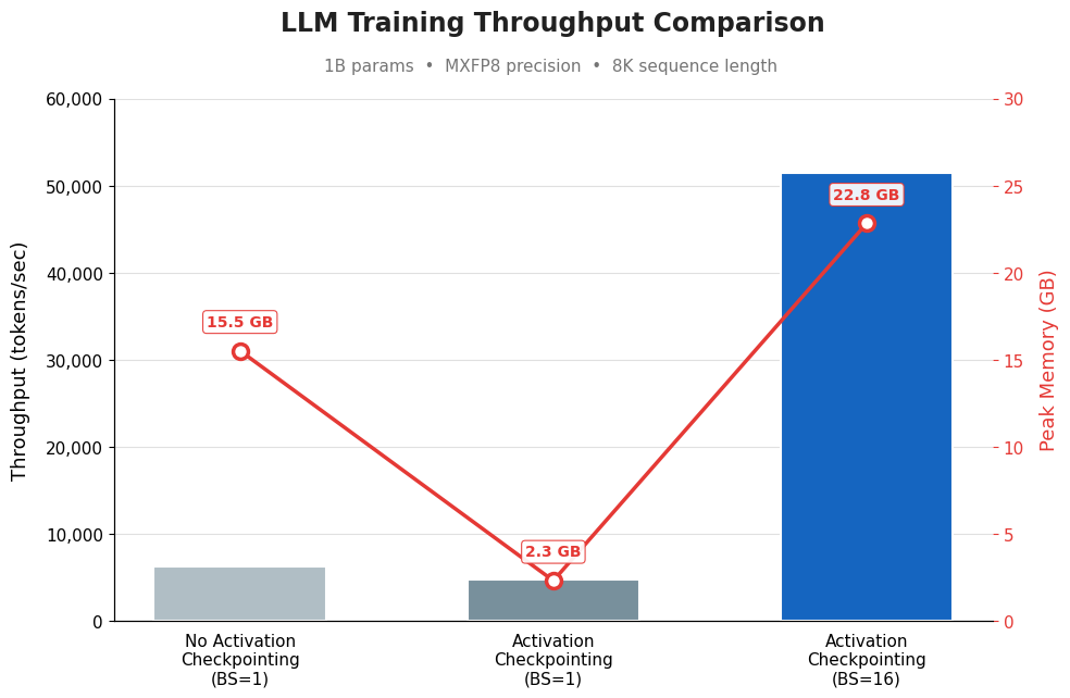
For example, in Figure 1, we compared three training configurations for a 1B-parameter LLM using MXFP8 precision at 8K sequence length. Without activation checkpointing (BS=1), throughput is ~6K tokens/sec but peak memory is high at 15.5 GB. Enabling activation checkpointing at the same batch size drops memory dramatically to 2.3 GB (since intermediate activations are recomputed instead of stored), but throughput also dips slightly because of that recomputation overhead. The key payoff comes in the third bar: with activation checkpointing enabled and batch size cranked up to 16, the freed memory allows a much larger batch, pushing throughput to ~51K tokens/sec (roughly 8x the baseline) while peak memory climbs to 22.8 GB, still well within GPU limits.

Figure 1. Throughput difference with and without activation checkpointing

To decide if activation checkpointing makes sense for your workload, consider your model size and memory usage:

Small models (up to ~14B parameters): Activation checkpointing is generally not needed. With Blackwell’s expanded memory, most small models fit comfortably without it. If you are running at the upper end of this range and hitting memory pressure, activation checkpointing adds compute overhead in exchange for meaningful memory savings, which you can reinvest into larger batch sizes.
Large models (~14B+ parameters): At this model size, memory consumption ranges from 87 to 171 GB depending on batch size and sequence length. Without activation checkpointing, most configurations fail with CUDA out-of-memory (OOM) errors. When you add checkpointing, the freed memory lets you increase batch size enough that throughput improves despite the added compute overhead. For large models, checkpointing is not optional. It is a prerequisite for stable training.

Precision formats

Blackwell’s fifth-generation Tensor Cores provide hardware acceleration for reduced-precision formats (FP8, MXFP8, and NVFP4), making them primarily throughput optimizations rather than memory-saving techniques. Using lower precision reduces memory bandwidth requirements, while also increasing the number of operations the GPU can run per cycle. However, reduced-precision training is roughly memory-neutral by default where Transformer Engine maintains both high-precision primary weights (for optimizer updates) and quantized copies, so lower precision formats don’t directly translate to lower memory usage. Quantization itself introduces overhead (converting between precision formats and maintaining multiple copies of weights in memory), which means the net benefit depends on model size and whether training is compute-bound or memory-bound. While NVFP4 offers the highest throughput, its performance benefits scale primarily with large models and inference workloads, where no primary weights are needed.

For compute-bound workloads (typically smaller models), calculation speed is the limiting factor, and quantization overhead partially offsets the throughput gains from lower precision. For memory-bound workloads (typically larger models), data movement is the bottleneck, and the reduced memory footprint of lower-precision formats directly addresses the constraint, delivering more significant gains:

Small models (up to ~14B parameters): At this model size, reduced-precision formats (FP8, MXFP8, NVFP4) all deliver similar, modest throughput improvements over FP16, since quantization overhead eats into the speed advantage. Batch size tuning tends to deliver more meaningful gains than precision format selection. Start with FP8 for higher throughput. It carries lower overhead than MXFP8 or NVFP4 and is often a good default for most small-model workloads. Note that with default TransformerEngine settings, reduced-precision formats use more memory than FP16, since TransformerEngine keeps weights in higher precision and casts them on-the-fly. If memory is a constraint and your optimizer supports it, use quantized_model_init to store weights directly in FP8, reducing memory below FP16 levels.
Large models (~14B+ parameters): This is where reduced precision delivers its greatest impact. FP8 typically provides a strong balance of throughput and memory efficiency. While MXFP8 is theoretically more memory-efficient, its transpose overhead partially offsets that advantage in practice. However, if convergence stability or numerical accuracy is a priority for your workload, MXFP8 may be the better choice, as its finer-grained quantization scheme tends to preserve model accuracy more reliably than FP8. For large models where memory is the primary bottleneck, NVFP4 can deliver additional throughput gains, as its matrix multiplication speed advantage scales with model size. Realizing those gains requires meaningful engineering investment. Use framework-level recipes from Megatron Core, which provide validated NVFP4 configurations, rather than implementing it from scratch.

NVIDIA’s TransformerEngine handles the implementation complexity: automatic mixed-precision switching, fused kernels, and dynamic loss scaling. Before moving to production, validate convergence by tracking loss curves across formats to confirm your chosen precision meets accuracy requirements.

Not every workload benefits from aggressive optimization. If your model trains comfortably within memory limits and meets your throughput requirements with FP16, the additional complexity of reduced-precision formats might not be worth the engineering effort. Start with baseline measurements, then optimize only the bottlenecks you can measure.

Getting started with Blackwell training on Amazon SageMaker AI

The preceding sections cover the key decisions: how much memory you have to work with, whether activation checkpointing makes sense for your model size, and which precision format fits your workload. The following sections put those decisions into practice using Amazon SageMaker AI training jobs.

Amazon SageMaker AI provides a fully managed environment for distributed training on Blackwell instances, handling instance provisioning, container orchestration, and integration with AWS services such as Amazon Simple Storage Service (Amazon S3), Amazon CloudWatch, Amazon Elastic Container Registry (Amazon ECR), and AWS Identity and Access Management (AWS IAM).

Prerequisites

Before you begin, confirm you have:

An AWS account with permissions to create Amazon SageMaker AI training jobs, access Amazon ECR, and create IAM roles for Amazon SageMaker AI execution.
Access to ml.p6-b200.48xlarge instances through a Flexible Training Plan or Managed Spot Training. Check your Service Quotas before starting.
Docker installed locally, Python 3.9 or later, and the SageMaker Python SDK.
Familiarity with PyTorch and FSDP. If you are new to FSDP, see Getting started with distributed training.

Launch a training job

To launch your training job, complete the following steps.

Step 1: Create your script

Download the fsdp.py file from the FSDP example from the NVIDIA TransformerEngine repository. This script implements FSDP training and accepts hyperparameters as command-line arguments.

Step 2: Create the entry point script

Prepare a train.sh file to configure torchrun and launch the training script:

#!/bin/bash

# SageMaker passes hyperparameters as environment variables (SM_HP_<NAME>)
PRECISION=${SM_HP_PRECISION:-"mxfp8"}
NUM_LAYERS=${SM_HP_NUM_LAYERS:-10}
BATCH_SIZE=${SM_HP_BATCH_SIZE:-8}
SEQ_LENGTH=${SM_HP_SEQ_LENGTH:-2048}

NUM_GPUS=$(nvidia-smi --list-gpus | wc -l)
torchrun --standalone --nnodes=1 --nproc-per-node="$NUM_GPUS" 
    fsdp.py --no-defer-init --precision "$PRECISION" 
    --num-layers "$NUM_LAYERS" --checkpoint-layer "transformerlayer" 
    --batch-size "$BATCH_SIZE" --seq-length "$SEQ_LENGTH"

Step 3: Build and push your container

Build a custom Docker container that extends the AWS Deep Learning Containers (DLC), includes fsdp.py and train.sh, and has TransformerEngine 2.11 installed. The DLC provides a validated base image with PyTorch and the CUDA libraries required for Blackwell compatibility. Here is the Dockerfile you can use:

FROM 763104351884.dkr.ecr.us-west-2.amazonaws.com/pytorch-training:2.9.0-gpu-py312-cu130-ubuntu22.04-sagemaker

# Install Transformer Engine
RUN pip install --upgrade --no-build-isolation transformer_engine[pytorch]==2.11.0
# Provide libcudart.so.12 for the pre-built flash-attn wheel
RUN pip install nvidia-cuda-runtime-cu12

# Make the linker able to find it
ENV LD_LIBRARY_PATH=/usr/local/lib/python3.12/site-packages/nvidia/cuda_runtime/lib:$LD_LIBRARY_PATH

COPY fsdp.py /opt/ml/code/fsdp.py
COPY train.sh /opt/ml/code/train.sh

ENV SAGEMAKER_SUBMIT_DIRECTORY /opt/ml/code
ENV SAGEMAKER_PROGRAM train.sh

Once built, create an Amazon ECR private repo if you do not already have one, and push the image to Amazon ECR (Note the repositoryUri from the output to use in the docker tag and push commands). For detailed build instructions, see Adapting your own Docker container to work with Amazon SageMaker AI.

Step 4: Secure capacity

Reserve capacity through a Flexible Training Plan for predictable access at the standard rate or use Managed Spot Training for cost-optimized workloads. Use Flexible Training Plans for production training runs requiring capacity reservation that is designed to provide continuous availability; use Spot for experimentation and fault-tolerant workloads where cost reduction outweighs the risk of interruption. Spot instances are subject to interruption, so make sure your training script saves checkpoints to Amazon S3 at regular intervals. Amazon SageMaker AI resumes an interrupted Spot job automatically if you provide a checkpoint_s3_uri in your estimator configuration. Create a Flexible Training Plan for predictable capacity on SageMaker AI console and select ‘training-job’ as the target resource. If your job can tolerate restarts and cost reduction is the priority, you can choose Spot, where you need to raise your quota for ml.p6-b200.48xlarge spot training job usage first. Note: Flexible Training Plans reserve capacity and incur charges for the duration of the plan, regardless of whether training jobs are actively running. Review pricing details before creating a plan.

Step 5: Submit the training job

Replace the placeholder values with your actual training plan ARN and ECR image URI, then run the following code from your local development environment or a SageMaker AI notebook instance:

from sagemaker.estimator import Estimator
from sagemaker import get_execution_role
from sagemaker.debugger import ProfilerConfig

training_plan_arn = "<your-training-plan-arn>"  # Replace with your training plan ARN
ecr_image = "<your-ecr-image-uri>"  # Replace with your ECR image URI

# Adjust these values to match your workload
precision = "mxfp8"
num_layers = 10
batch_size = 8
seq_length = 2048

estimator = Estimator(
    image_uri=ecr_image,
    role=get_execution_role(),
    base_job_name='blackwell-training',
    instance_count=1,
    instance_type='ml.p6-b200.48xlarge',
    hyperparameters={
        "precision": precision,
        "num-layers": num_layers,
        "batch-size": batch_size,
        "seq-length": seq_length,
    },
    profiler_config=ProfilerConfig(disable_profiler=True),
    training_plan=training_plan_arn)

estimator.fit()

For Managed Spot Training, replace training_plan with use_spot_instances=True, set max_run and max_wait, and add a checkpoint_s3_uri for automatic resumption.

Step 6: Monitor your training job

Amazon SageMaker AI streams logs to Amazon CloudWatch automatically. In the SageMaker AI console, navigate to Training jobs and select your job to find the CloudWatch log group. Open /aws/sagemaker/TrainingJobs and look for [rank 0] lines for loss values and throughput. To confirm your precision format loaded, look for messages such as “Using FP8 recipe” or “MXFP8 enabled”.

If your job stops with a CUDA out-of-memory (OOM) error, the log shows the allocation size. Reduce batch size or sequence length or add activation checkpointing if you have not already done so.

Cleanup

To avoid ongoing charges after your tests, stop any running training jobs in the Amazon SageMaker AI console (note that this does not cancel a Flexible Training Plan). Warning: The following cleanup steps permanently delete resources and cannot be undone. Verify you have backed up any data you need before proceeding. Delete your Amazon ECR repository (this permanently removes container images), delete any training artifacts stored in Amazon S3 (this permanently removes training data and checkpoints), and remove the CloudWatch log groups (this permanently removes training logs). Delete the IAM execution role created for Amazon SageMaker AI.

Conclusion

In this post, you learned how to optimize AI model training on NVIDIA Blackwell GPUs using Amazon SageMaker AI training jobs. You configured batch sizes and sequence lengths to take advantage of Blackwell’s expanded memory, applied activation checkpointing based on your model size, and selected precision formats suited to your workload. You also set up a custom container with TransformerEngine, secured capacity through a Flexible Training Plan, and launched a distributed training job on ml.p6-b200.48xlarge instances.

Transformer models from 1B to 64B parameters show consistent gains when you combine these optimizations. The key is understanding whether your workload is compute-bound or memory-bound, then applying changes incrementally so you can measure the impact of each one.

If you are ready to get started, explore the Amazon SageMaker AI documentation to review instance options and configuration details, or purchase a Flexible Training Plan to reserve Blackwell capacity for your next training run. If you have questions about your specific workload, contact AWS Support or your AWS account team.